[전국 도시 공원 표준 데이터] 시도별 공원 분포

4. 시도별 공원 분포

 

4.1 시도별 공원 비율

 

• 시도별로 합계 데이터 출력

city_count = df["시도"].value_counts().to_frame()
city_mean = df["시도"].value_counts(normalize=True).to_frame()

  - normalize=True : 비율로 구하기

  - 둘을 합쳐주기 위해 dataframe 형태로 바꾸었다.

 

 

 

 

 

• 합계와 비율 함께 구하기: merge

city = city_count.merge(city_mean, left_index=True, right_index=True)
city.columns = ["합계", "비율"]
city.style.background_gradient()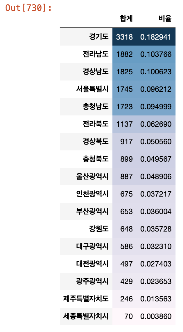

 

 

 

 

---

 

 

4.2 공원구분별 분포

 

• "공원구분" 별로 색상 다르게, "공원면적" 별로 원의 크기 다르게

plt.figure(figsize=(8, 9))
sns.scatterplot(data=df_park, x="경도", y="위도", hue="공원구분", size="공원면적", sizes=(10, 100))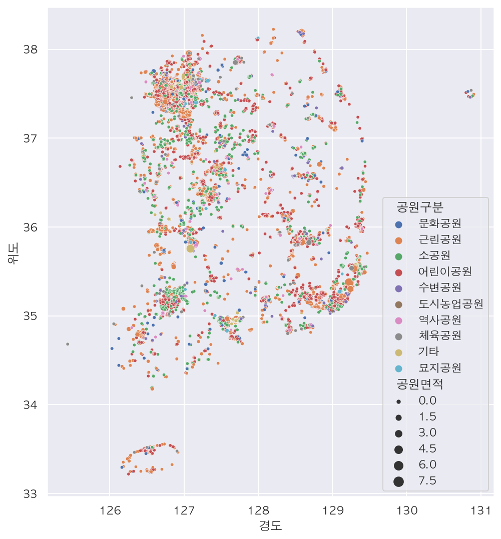

 

 

 

 

 

---

 

 

4.3 시도별 공원분포

 

• "시도" 별로 색상 다르게, "공원면적" 별로 원의 크기 다르게

plt.figure(figsize=(8, 9))
sns.scatterplot(data=df_park, x="경도", y="위도", hue="시도", size="공원면적", sizes=(10, 100))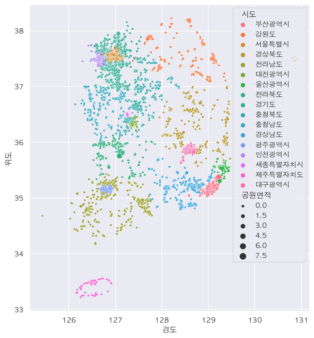

 

 

 

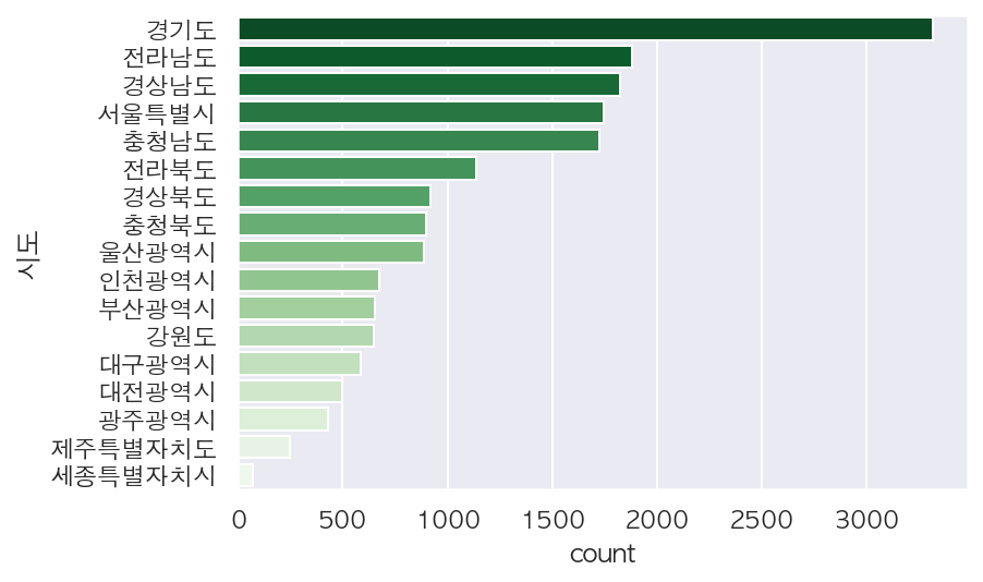
• countplot 으로 시도별 빈도수 그리기

sns.countplot(data=df, y="시도", order=city_count.index, palette="Greens_r")